
Goals
- To develop an intuitive understanding of the how the General Linear Model (GLM) is used for univariate, single-subject, single-run fMRI data analysis
- To understand the significance of beta weights in GLM analysis
- To understand the significance of residuals in GLM analysis
- To learn to perform single-subject GLM analysis in BrainVoyager
- To learn to interpret statistical analysis of beta weights
Relevant Lectures
General Linear Model
Accompanying Data
I. Applying the GLM to Single Voxel Time Courses
The General Linear Model (GLM) is a fundamental statistical tool that is widely applied to fMRI data. In this tutorial, you will learn the basics modelling BOLD activation time courses using the GLM. First, we will explore how GLM analysis works one voxel at a time. Then we will move to BrainVoyager to do the analysis and apply statistical maps over an entire volume.
Recall that the GLM is used to model data using the form y = β0 + β1X1 + β2X2 + ... + βnXn + e where y is the observed or recorded data, β0 is a constant or intercept adjustment, β1 ... βn are the beta weights or scaling factors, and X1 ... Xn are the independent variables or predictors.
Alternatively, if you're not into matrix algebra, you can think of this as modelling a data series (time course) with a combination of predictor time courses, each scaled by beta weights, plus the "junk" time course (residuals) that is left over once you've modelled as much of the variance as you can.
In fMRI data analysis, whether we are looking at a single voxel, the average of all voxels within a specific region, or each and every voxel in the brain, we want to do two things. First, we want to provide a mathematical estimate of how active the voxel is for each of our conditions. Second, we want to test whether differences between conditions are statistically significant.
Let's first consider the simplest possible example: one run from one participant with two conditions. Note that we always need at least two conditions so that we can examine differences between conditions using subtraction logic. This is because measures of the BOLD signal in a single condition are affected not only by neural activation levels but also by extraneous physical factors (e.g., the coil sensitivity profile) and biological factors (e.g., the vascularization of an area). As such, we always need to compare conditions to look at neural activation (indirectly) while subtracting out other factors.
In the following plot, a simulated 'data' time course is shown in grey, and is presented in arbitrary units over time in seconds (here we had a 1-s TR so seconds = volumes). There is also a single predictor X1 shown in pink. The predictor can be multiplied by a beta weight and a constant can be added, using the sliders. To get a residual time course (lower panel), we subtract the predictor/model from our data at each point in time. The goodness of fit between the data and the model can be computed as the squared error, also called the sum of squared residuals.

Note: In case that the following plot shows up white without showing any data please check on your browser that the script is "allowed/unblocked". Usually it will give you a little notifaction on the website URL. It might look similar to the image to the right (Chrome). If this is the case click "load unsafe script".
Adjust the sliders until you find the beta weight and constant that best fit the data.
Note: The web formatting is a bit wonky so you may have to scroll left-right in the window below to see different parts of the window (we'll try to fix this soon).
Question 1: How can you tell when you've chosen the best possible beta weight and constant -- Consider (1) the similarity of the weighted predicted (purple) and the data (black) in the top panel; (2) the appearance of the residual plot in the bottom panel; and (3) the squared error and sum of residuals? How does the beta weight affect the weighted predictor? What percentage of the total variance would the best model account for? What aspects of the data might adjustments of the beta weight NOT affect that may still affect the goodness of fit of the residuals? How does changing the constant affect the model? In practice, we don't expect to find a perfect fit between predictors and data. The following is a more realistic example with noisy data.
Adjust the sliders in the following plot to find the best fit between the predictor and the data.
Question 2: What values did you choose? What are the resulting error and sum of residual? How do the residuals and squared error differ in this case compared to the first case? In fMRI analysis, we are usually interested in explaining signal variance in terms of multiple experimental conditions, not just a single one. The following examples use data taken from the course dataset — a 2 condition + baseline variant of the localizer sessions. The participant was shown images of faces and hands in alternating 16-s blocks. The timecourses from three voxels were extracted, and two task-specific predictors were generated according to the block design. No preprocessing was applied.
adjust the heights of beta1 and beta2
Convolve button
Question 3: Based on the effect of convolution on your predictors, which type of Hemodynamic Response Function was employed in the convolution?
Adjust the sliders until you think you have optimized the model (i.e., minimized the squared error). Make sure you understand the effect that the two betas and the constant are having on your model. You can test how well you did by clicking the Optimize GLM button, which will find the mathematically ideal solution.
Question 4a: What can you conclude about Voxel 1's selectivity for images of faces and/or hands? Where in the time course do the residuals deviate the most from the model? Why?
Repeat the optimization process for Voxel 2.
Question 4b: What can you conclude about these Voxel 2's selectivity for images of faces and/or hands?
Repeat the optimization process for Voxel 3.
Question 4c: What can you conclude about Voxel 3's selectivity for images of faces and/or hands? What does it mean if a beta weight is negative?
Question 5: Define what a beta weight is and what it is not.
II. Whole-brain Voxelwise GLM in BrainVoyager

Now you should understand how the GLM can be used to model data in a single voxel, but we have over 300,000 voxels in our data set. How can we get the bigger picture? One way is to do a whole-brain voxelwise GLM. "Voxelwise" means that we run not just one GLM but one GLM for every voxel. This is sometimes also called a "whole-brain" analysis because typically the scanned volume encompasses the entire brain (although this is not necessarily the case, for example if a researcher scanned only part of the brain at high spatial resolution).
1) Open BrainVoyager , then Open, navigate to the BrainVoyager Data folder, then select and open P1_anat-S1-BRAIN_IIHC_MNI.vmr
2) Select the Analysis menu and click Protocol… Next, in the Protocol window, click the Load .PRT... button. Select and open Run01.prt from the PRTs folder. You should now see Face and Hand in the Conditions list. Click the Close button.
3) Click the Analysis menu again, this time selecting Link Volume Time Course (VTC) File ... In the window that opens, click Browse then select and open P1_Run1_S1R1_MNI.vtc , then click OK.

You have now loaded all three files: the anatomical volume, the functional data, and the experimental protocol that BrainVoyager will use for GLM analysis.
4) Now, let’s get started with the GLM analysis. Click the Analysis menu and select General Linear Model: Single Study. By single study, BrainVoyager means that we will be applying the GLM to a single run.
Click options and make sure that Exclude first condition ("Rest") is unchecked (the default seems to be that it is checked). Click Define Preds to define the predictors in terms of the PRT file opened earlier and tick the Show All checkbox to visualize them. Notice the shape of the predictors – they are identical to the ones we used earlier for Question 3. Now click GO to compute the GLM in all the voxels in our functional data set.

After the GLM has been fit, you should see a statistical "heat-map" overlaid on the anatomical scan (but remember the map was generated from the functional scans). This initial map defaults to showing us statistical differences between the average of all conditions vs. the baseline. More on this later.
Note: If you want the maps in your Verstion of BrainVoyager to match the appearance of those in the tutorials, in BrainVoyager Preferences (BrainVoyager/Preferences on Mac), in the GUI panel, turn off Dark mode and change the Default Map Look-up Table to "Classic Map Colors (pre-v21)".

In order to create this heat map, BrainVoyager has computed the optimal beta weights at each voxel such that, when multiplied with the predictors, maximal variance in the BOLD signal is explained (under certain assumptions made by the model). Another, equivalent interpretation, is that BrainVoyager is computing beta weights that minimize the residuals. For each voxel, we then ask, “How well does our model of expected activation fit the observed data?” – which we can answer by computing the ratio of explained to unexplained variance.

It is important to understand that, in our example, BrainVoyager is computing two beta weights for each voxel – one for the Face predictor, and one for the Hand predictor. And for each voxel, residuals are obtained by computing the difference between the observed signal, and the modelled or predicted signal – which is simply vertically scaled by the beta weights. This is the same as you did manually in Question 3.
But we don't simply want to estimate activation levels for each condition by computing beta weights; we also want to be able to tell if activation levels differ statistically between conditions!
Just as with statistics on other data (such as behavioral data), we can use the same types of statistics (e.g, t-tests, ANOVAs) to understand brain activation differences and the choice of test depends on our experimental design (e.g., use a t-test to compare two conditions; use an ANOVA to compare multiple conditions or factorial designs). Statistics provides a way to determine how reliable the differences between conditions are, taking into account how noisy our data are. For fMRI data on single participants, we can estimate how noisy our data are based on the residuals.
For example, we can use a hypothesis test to test whether activation for the Face condition (i.e., the beta weight for Faces) is significantly higher than for Hands (i.e., the beta weight for Hands). Informally, for each voxel we ask, “Was activation for faces significantly higher than activation for hands?”
To answer this, it is insufficient to consider the beta weights alone. We also need to consider how noisy the data is, as reflected by the residuals. Intuitively, we can expect that the relationship between beta weights is more accurate when the residuals are small.
Question 6: Why can we be more confident about the relationship between beta weights when the residual is small? If the residual were 0 at all time points, what would this say about our model, and about the beta weights? Think about this in terms of the examples in Questions 1,2 and 4.
We can perform these kind of hypothesis tests using contrasts . Contrasts allow you to specify the relationship between beta weights you want to test.

5) From the Analysis menu, select Overlay General Linear Model... then click the box next to Predictor 2 until it changes to [-] you also want to make sure that Predictor 1 is set to [+] .
Note: In BrainVoyager, the Face and Hand predictor labels appear black while the Constant predictor label appears gray. This is because we are not usually interested in the value of the Constant predictor so it is something we can call a "predictor of no interest" and it is grayed out to make it less salient. Later, we'll see other predictors like this.
Question 7: In the lecture, we discussed contrast vectors. What is the contrast vector for the contrast you just specified?
Click OK to apply the contrast. Use the mouse to move around in the brain and search for hotspots of activation.
By doing this, you are specifying a hypothesis test to test whether the beta weight for Faces is significantly different (and greater than) the beta weight for Hands. This hypothesis test will be applied over all voxels, and the resulting t-statistic and p-value (error probability value) determine the colour intensity in the resulting heat map.
Question 8: Can you find any blobs that may correspond to the fusiform face area or the hand-selective region of the lateral occipitotemporal cortex?
This heatmap is generated using a t-statistic at each voxel (and a corresponding p-value).

6) Locate Overlay Volume Maps under the Analysis tab. Click it and you will see a GUI appear. Alternate between checking and unchecking Trilinear Interpolation and look at how the colour map changes on the brain.
Question 9: What effect does Trilinear Interpolation have on the map? Which way of viewing the map is more true to the data that was used to generate the statistical map and which way is "prettier"?
Next check the Trilinear Interpolation again and click Close.

7) Use the Decrease Threshold and Increase Threshold buttons on the left-hand side of the main window to adjust the p-value threshold of this contrast. Decrease the threshold until nearly every voxel has been coloured in.
Question 10: What is the p-value for this threshold? What does this map show us? How can you interpret the colours in this heatmap – does a voxel being coloured in orange-yellow vs. blue-green tell you anything about how much it activates to Faces vs. Hands?
III. Corrections for Multiple Comparisons
Our whole-brain voxelwise analyses have revealed which voxels are most statistically reliable, but how will we determine which p-value cut-off (threshold) to use, especially considering that the GLM was run on over 300,000 voxels. Let's explore different options.
8) Let's start with the usual convention, p < .05.
On the Statistic tab (Analysis/Overlay volume map), click Use statistic value. Then on the Map Options tab, set p-value to .05 and click Apply.

Question 11: Given that a p-value threshold of .05 is the usual statistical standard, why is it suboptimal for voxelwise fMRI analyses?
9) Now let's try applying a Bonferroni correction. Under Map Options, ensure the p-value is set to .05 but this time, check the Bonferroni box and click Apply.
Question 12: What do you see on the map? Can you find any activation that survived this correction?
10) Now let's look at the effects of applying a cluster correction. Generally, cluster corrections should only be used with a p-value threshold -- here called a cluster-determining threshold -- of 0.001 or stricter. Turn off Bonferroni correction and set the p-value to 0.001. Look at the map to remember how it looks.
We ran a plug-in in BrainVoyager to compute the likelihood of getting clusters of different sizes in 1000 randomly generated data sets where no legitimate differences between conditions were present. Here is the output:

This output shows the probability of finding clusters of different sizes when no such effect is actually present (i.e., Type I errors).
Question 13: Based on this output, what is the appropriate cluster size for cluster correction?
Enable cluster thresholding (in the statistics tab) and ensure the number of voxels matches the cutoff you determined.

11) Lastly, let's examine a False Discovery Rate correction.
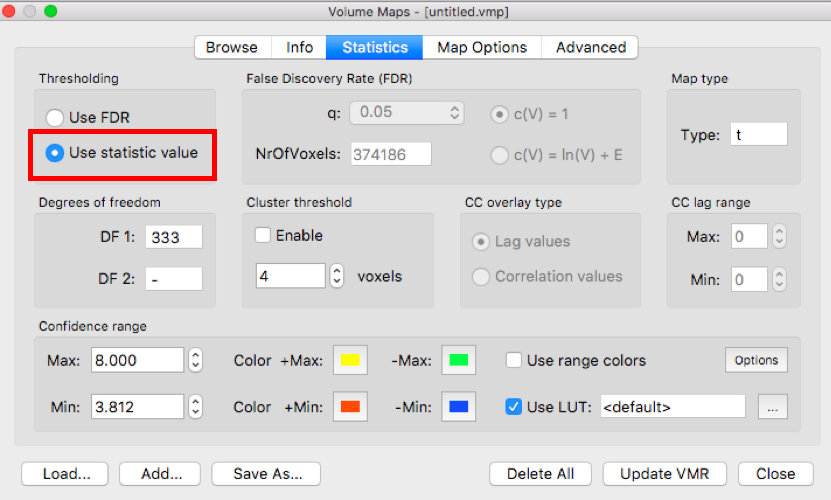
In the Statistics tab, turn on Use FDR.

Question 14: You've now examined the following cases: (a) uncorrected p .05; (b) Bonferroni-corrected p .05; (c) cluster threshold correction; and (d) false-discovery-rate correction. In your view, which approach(es) is/are best and why?